This page gives you a guided tour of the SIRA_PRISE DML language, in a sort of learn-by-example kind of way. It has three main sections : Query basics, advanced relational algebra operators, and updating. All examples used on this page are available for copy-paste in this text file.
Started up the server ?
Then we will get you started with writing SIRA_PRISE expressions involving relvars, renames, projections, relation intersections, relation differences, relation unions, various join operators, relation extends and relation restrictions. Followed by a section on ordering results.
Querying relvars.
Now start up either the DBrowser or a web browser (in which case also point it to your web app server, its SIRA_PRISE web app, and choose the console function). Connect to localhost or 127.0.0.1, port 50000, and enter
RELVAR
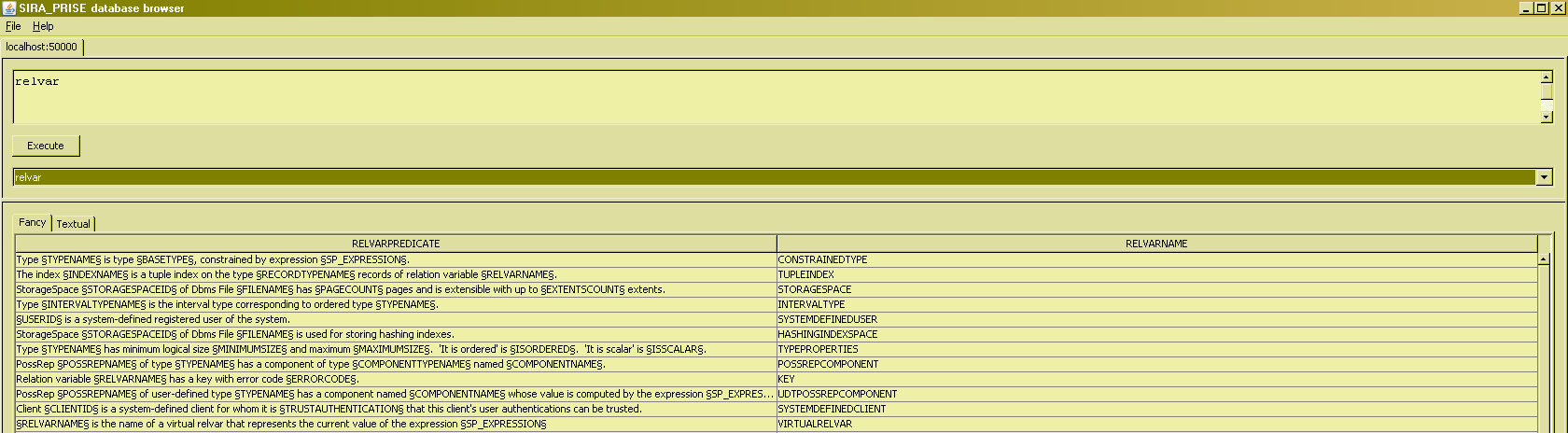
Congratulations ! You have successfully issued your first SIRA_PRISE query. Your client has just sent "INQUIRE relvar" to the server, gotten the stream of bytes you can inspect under the tab "Textual" in reply, and used that to format the data in the "Fancy" tabular form shown above. Note that while in the DBrowser and the web client console, you can suffice with typing just the expression you want, doing a query in the script processor will require to spell the command out in full : INQUIRE <RelationalExpression>, that is.
Anyhow, it seems that the word "relvar" is a valid <RelationalExpression>, apparently. You will have guessed that one particular kind of <RelationalExpression> is to just name an existing relvar, and that "relvar" is one such. The contents listed show you all base relvars that exist in the database, so ... anything listed under the heading "relvarname" should give a valid executable query in turn ... Let's check that out ...
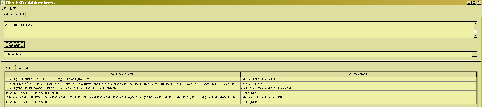
What you see here is an overview of all the virtual relvars that exist in the database, and since virtual relvars can be used as any other relvar (ducking the issue of view updating at this point), once again anything listed under the heading "relvarname" should give a valid executable query in turn ... Let's check that out ...
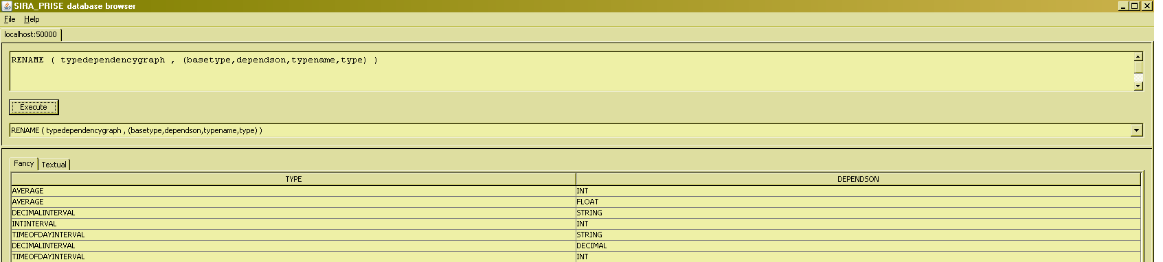
RENAME
Okay ... Now we know how to get to the relvar names we can query, how do we write expressions of the relational algebra referencing those relvars ??? Knowing just a few basic principles of SIRA_PRISE syntax will help you do exactly that.
- All invocations of RA operators are to be specified in prefix notation, that is, the same way you are probably used to when you need to compute the cosine of a value : COS( <argument here> ). Thus, all RA invcoations in SIRA_PRISE take on the syntactic form OP( <arguments here> ).
- The arguments in the argument list are separated by a comma
- Relation-typed arguments can of course themselves be some other RA operator invocation, iow, RA operator invocations can be nested.
- Certain operators take "arguments" that aren't relational expressions, but certain kind of "lists of stuff". Syntactically, that list is always enclosed in parentheses. Some operators to which this applies are RENAME, PROJECT, EXTEND, SUMMARIZE, GROUP, ... Such operator invocations thus always take on the form OP ( <rel arg here> , ( <list arg here> )).
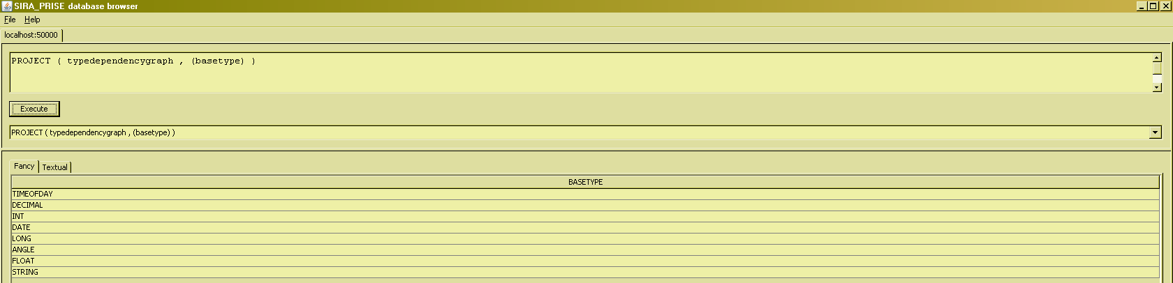
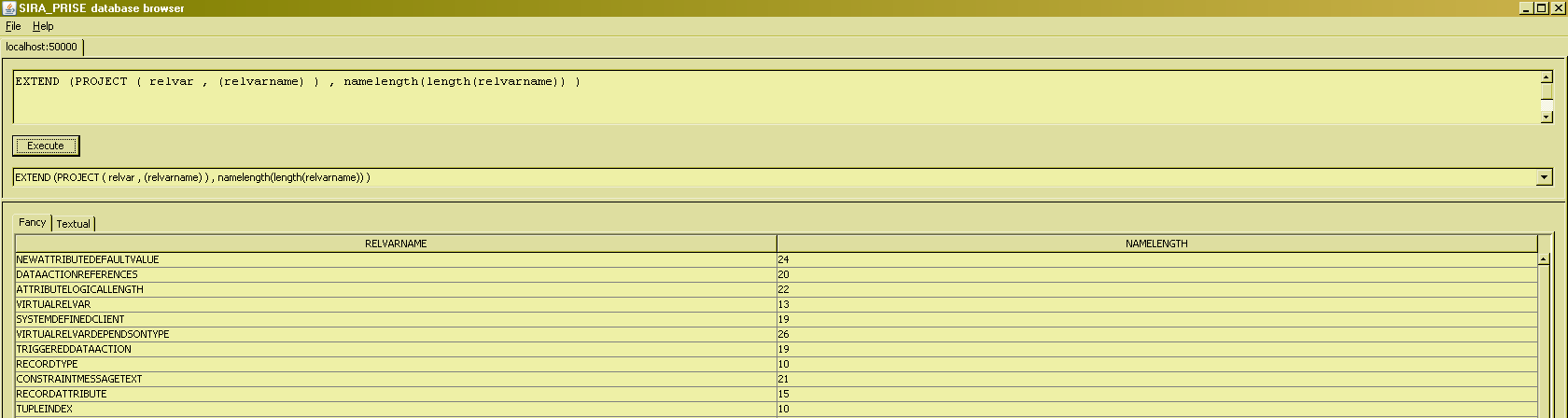
PROJECT
It will not be very hard to guess at this point what a PROJECTion will look like syntactically :
INTERSECT
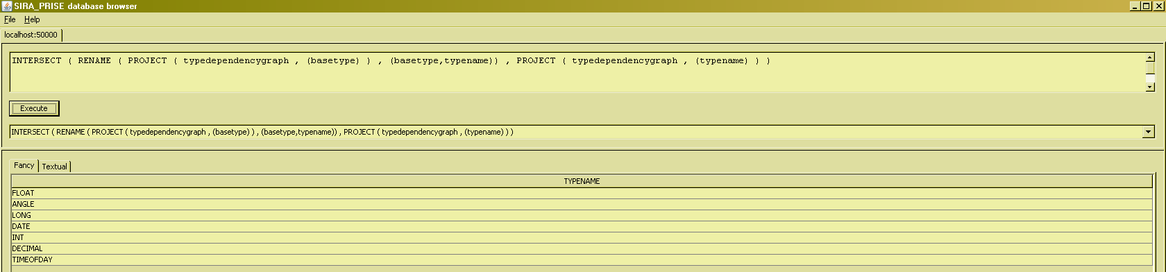
Knowing how to write projections and renames, we can use these to start writing queries that involve the basic "set" operations of the relational algebra. E.g. to answer the question "which types are both dependent upon some other type and required for some [yet other] type ? To answer that, we will need INTERSECTion :
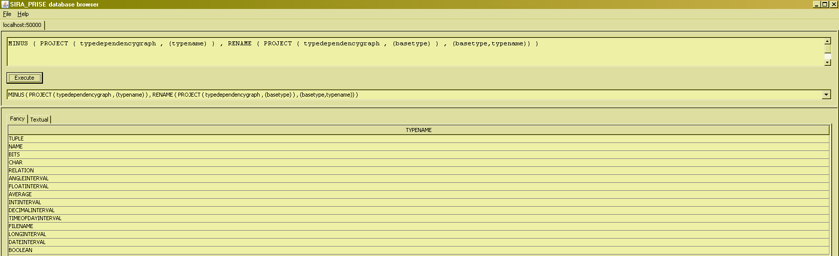
MINUS
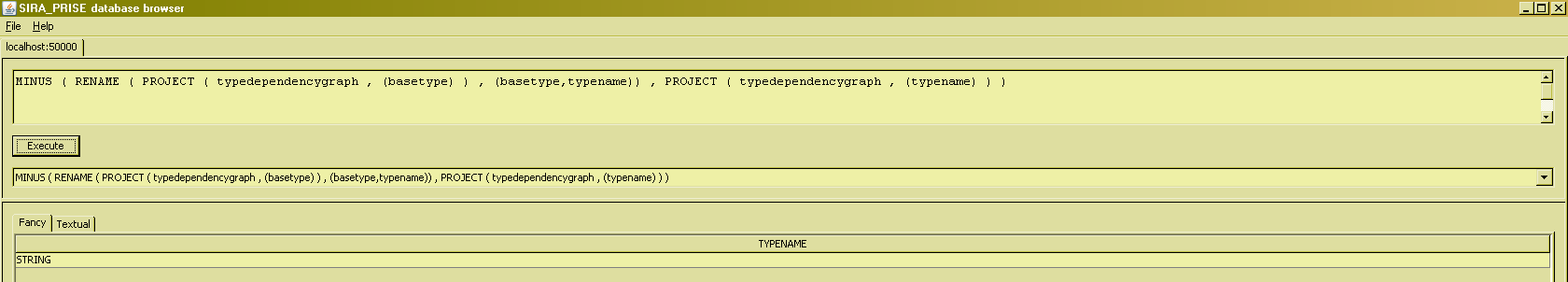
Similar questions are : "Which types depend on other types for their definition, but are themselves not required for the definition of other types ?" and "Which types are required for the definition of other types, but are themselves not dependent on other types for their own definition?" . These questions can be answered using the (most basic) difference operator of the relational algebra, MINUS :
UNION
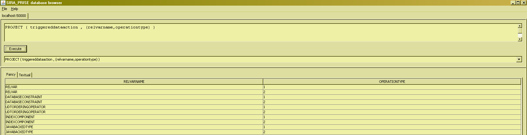
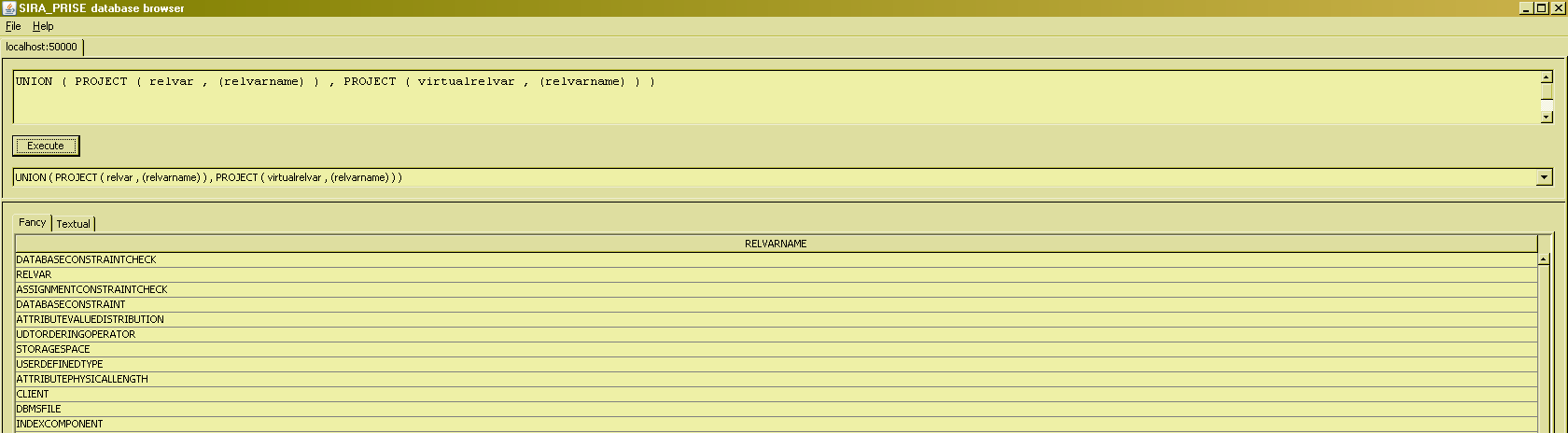
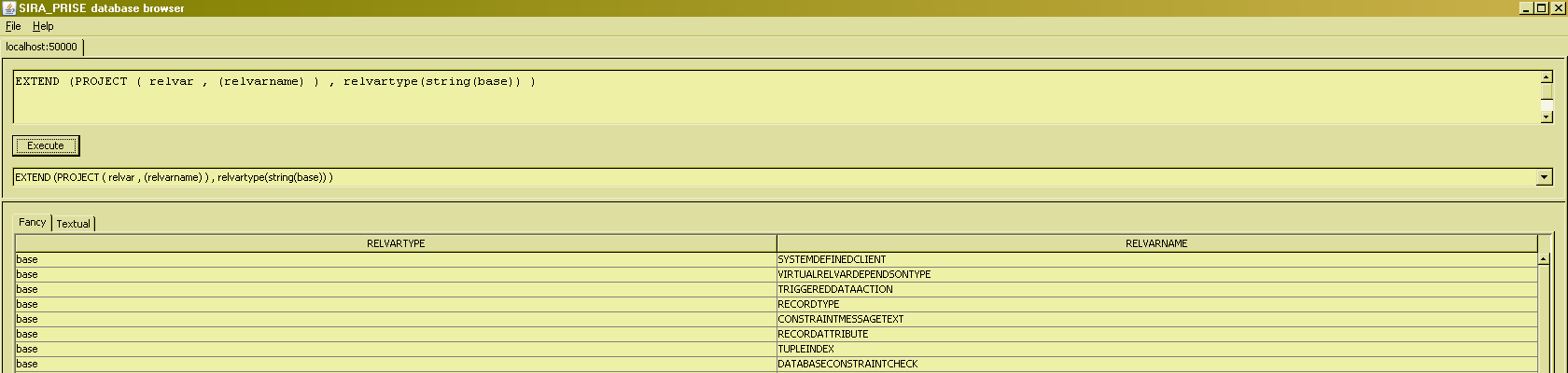
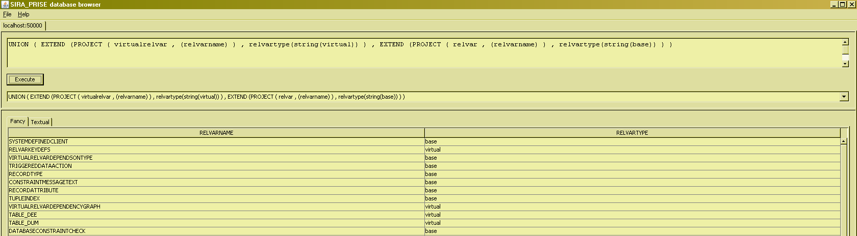
The last remaining operator of the "basic set operations" of the relational algebra is UNION. We can use it to answer questions like "What are all the relvars known to the system ?" :
JOIN
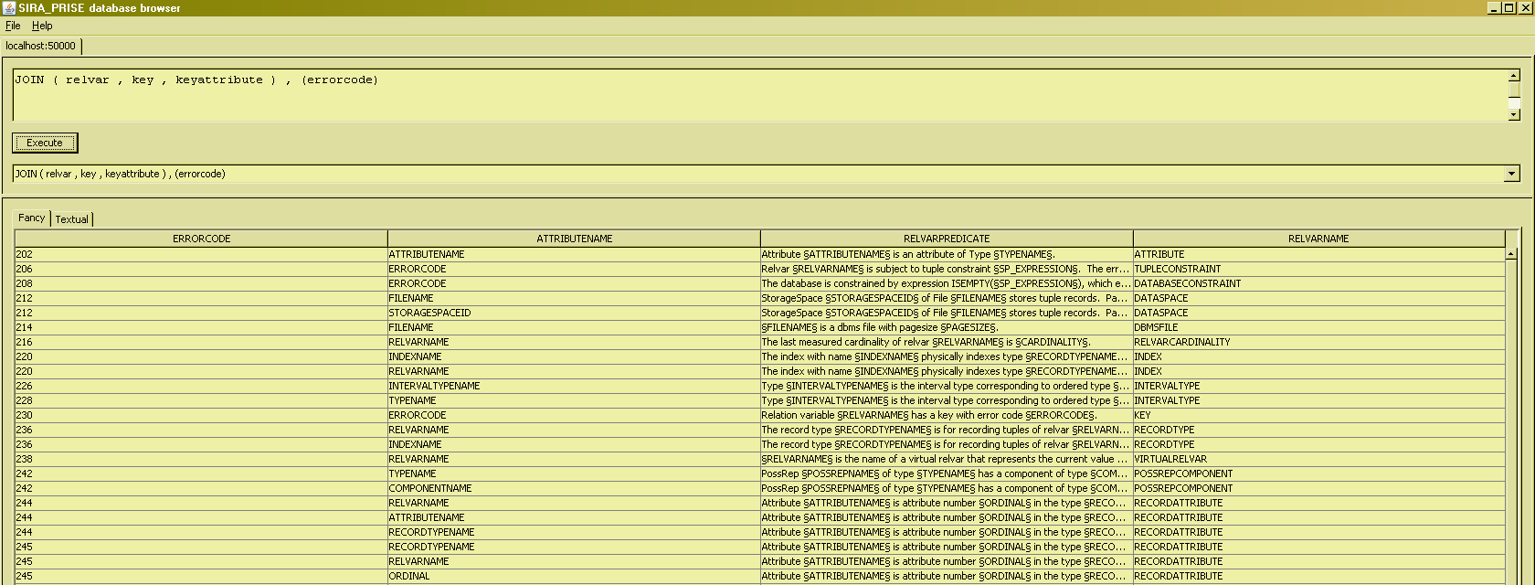
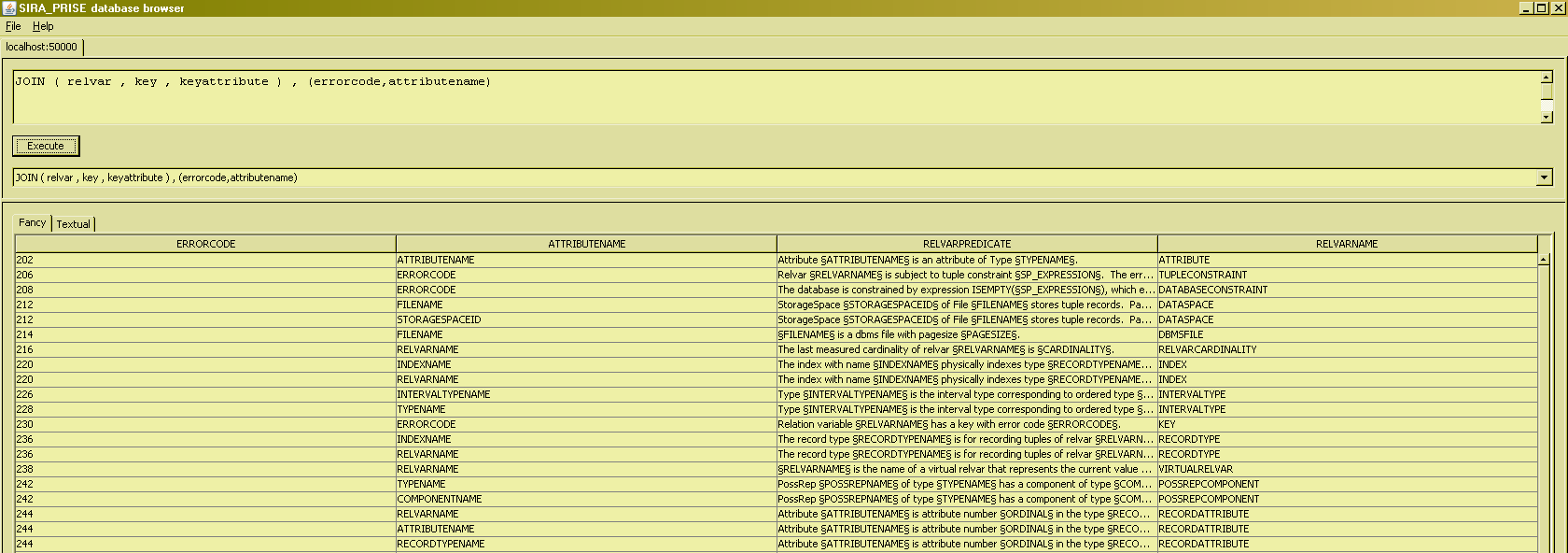
Next operator you are by now probably itching to try out is JOIN (and relatives). At this point, and in order to make it a bit easier to understand the examples given here, it might be interesting to first take a look at the values (and the headings) of the relvars used here : RELVAR, KEY, and KEYATTRIBUTE. E.g. to answer "Which are the relvars for which a key is defined, and which key is that ?", we could use a natural join, the syntax for which is simple and straightforward :
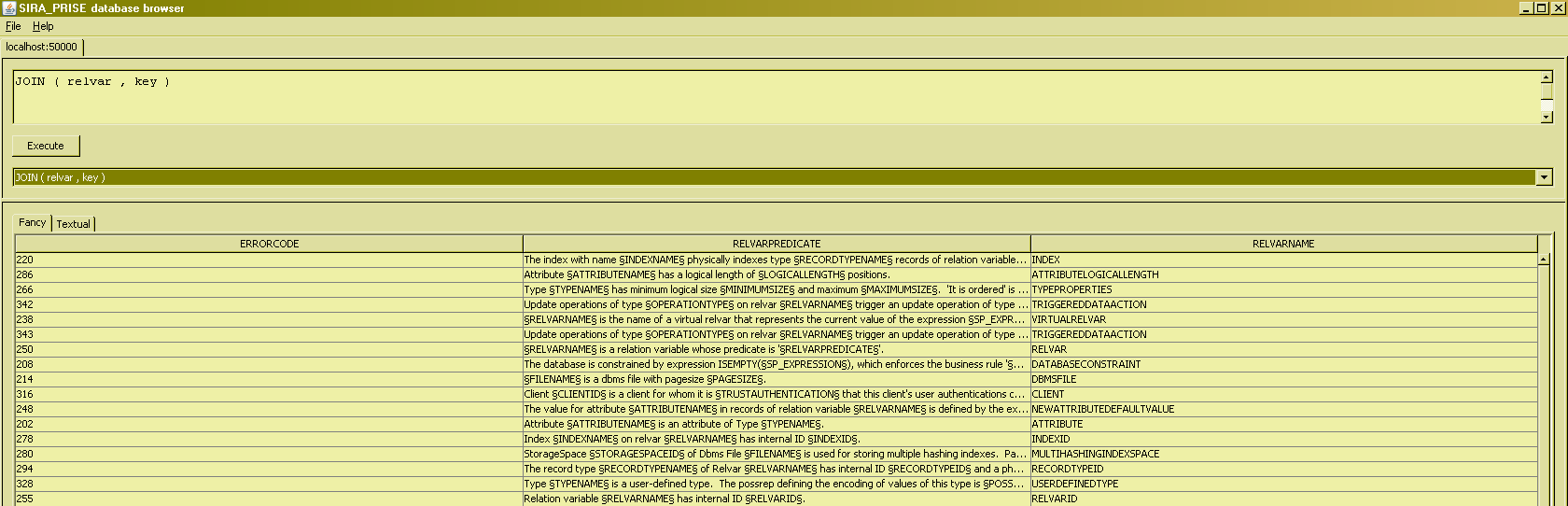
All in all, we're not really much wiser after having seen this, are we ? What we're really interested in is knowing what the attributes are that constitute any key, of course. We can do this by joining in the relvar that holds this info, and because JOIN is an associative operator, we do not need to
nest dyadic invocations, but we can suffice writing the three-relvar JOIN simply as :
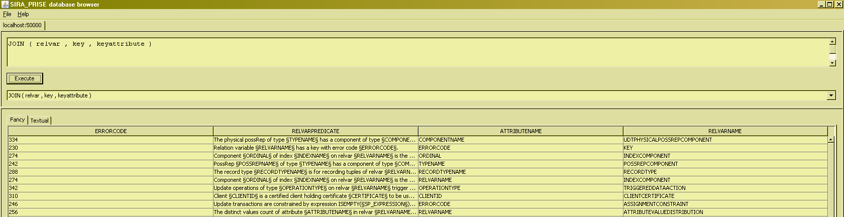
Observe that the lines are "scattered all over the place", e.g. both the third and sixth line mention an attribute of a key to the relvar named "indexcomponent", with lines regarding completely other relvars intermitting. This is in keeping with the principle that there is no inherent ordering to the tuples that appear in a relation. Matters of ordering and grouping together will be addressed later.
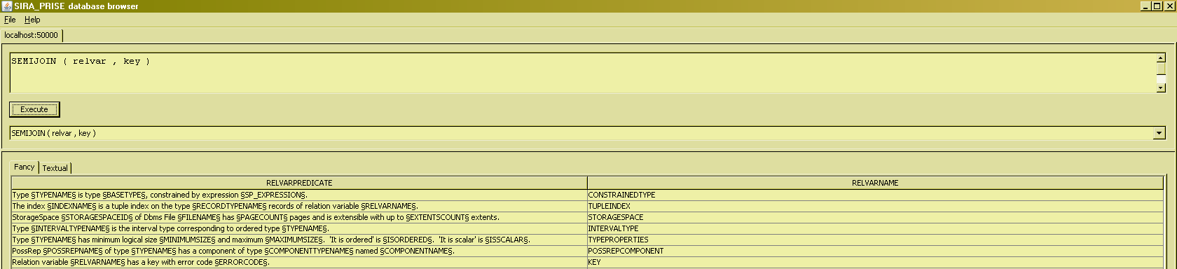
SEMIJOIN
Natural join has the properties that :
- The resulting relation includes all the attributes that appear in any of the arguments to the join,
- The resulting relation includes only tuples for which "matching values" appear in all the arguments to the join.
SEMIMINUS
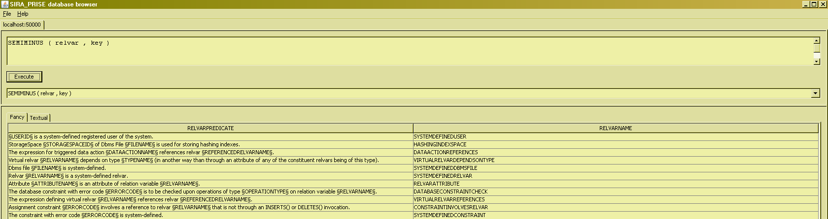
Observe that the resulting list is a bit shorter than the one we got from our very first query, which was just to list all (base) relvars. This clearly suggests that there are some (base) relvars for which no key is defined at all, and often the question is precisely to figure which ones those are ... Now naturally, you could apply the MINUS operator to the "full" list and the semijoin just given, but because this kind of query is so often needed in practice, a shortcut called SEMIMINUS is provided that does exactly that (those who follow Tutorial D will know this operator as NOT MATCHING) :
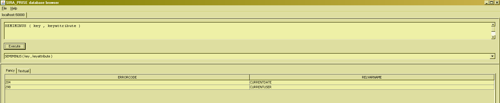
A very similar query would be "What are the keys that have no attribute at all ?". For those to whom this seems a bit alien : yes, that's a perfectly sensible question. Keys on a relvar can indeed be on no attributes at all, thereby constraining the relvar to hold at most one tuple at any time. The question at hand is answered by :
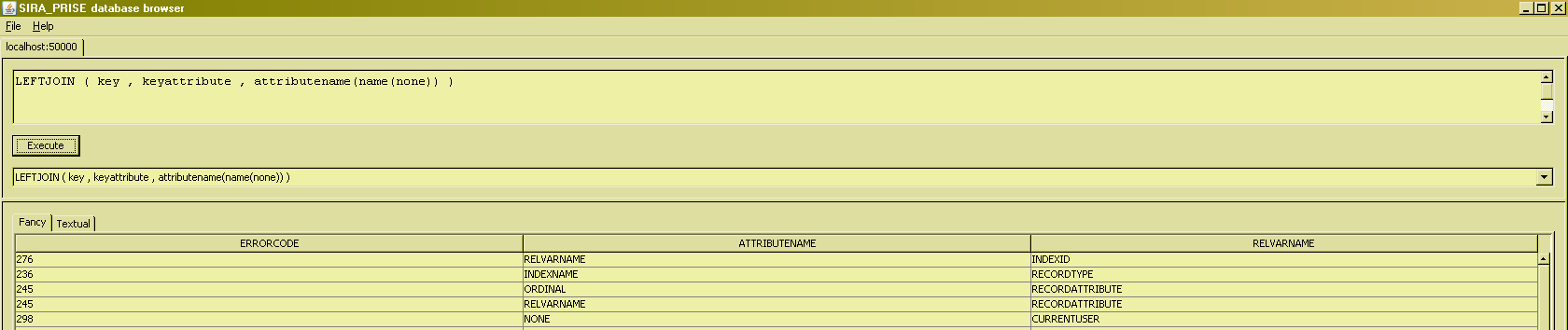
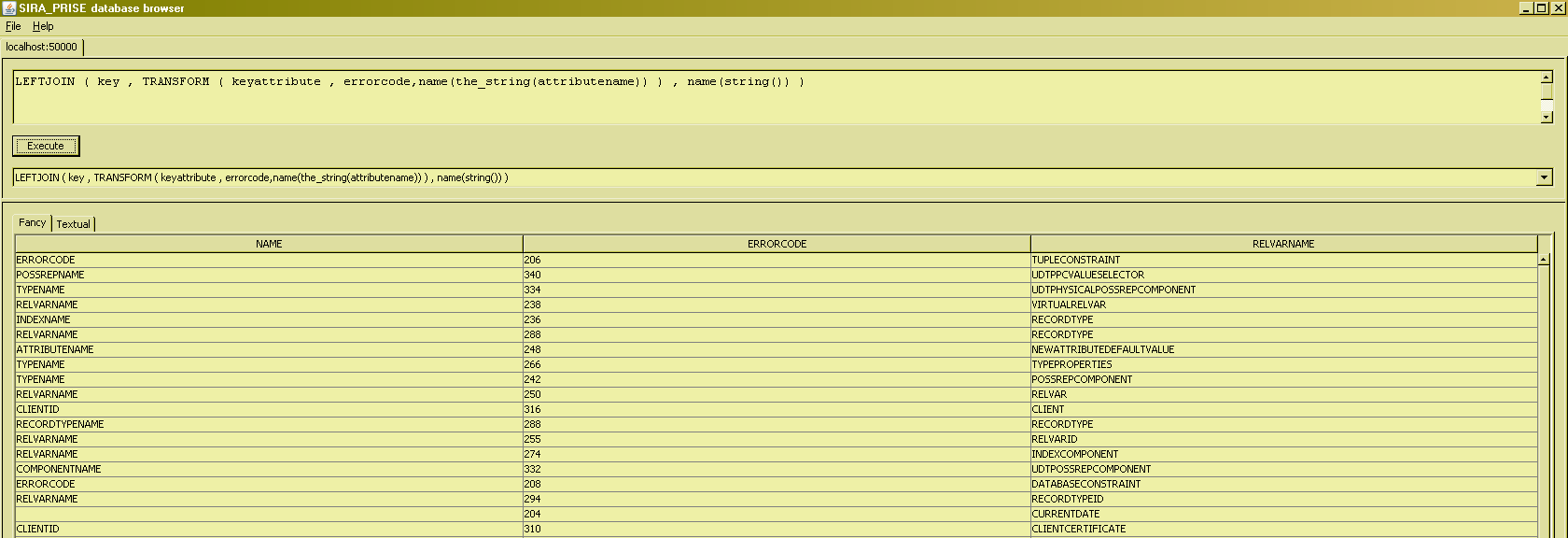
LEFTJOIN
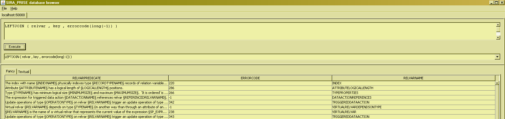
So now what if we want to obtain an overview of all keys, mentioning their attributes, but we also want a mention of the keys that have no corresponding attributes ? We obviously can't use JOIN or SEMIJOIN, as those would eliminate keys 204 and 298 from the result set. And we also cannot simply take a JOIN query and a SEMIMINUS query, and UNION the two together, because the headings of the results returned by those two queries are not identical ... And unlike in SQL, null cannot come to the rescue because we obviously want to stay within the bounds of the relational model ...
LEFTJOIN offers some kind of solution, allowing us to get out of this apparent stalemate. LEFTJOIN is much like SQL's outer join, but where SQL would otherwise place nulls in the result, LEFTJOIN requires the user to provide a genuine value of the concerned attribute type to place in the result. In some cases, this can suffice as a solution (ex. 1), in other cases, it is obvious that this is still not much more than an ugly hack (ex. 2).
Example 1 answers the question "List all the relvars and the identifying number of the keys declared on them, using the number -1 if no key is defined.". This "hack" won't be that unfamiliar. Negative numbers are often used for such a purpose if and when "genuine" values will always be strictly positive.
EXTEND
The last two basic operators to be discussed are RESTRICT and EXTEND. Both involve "arguments" that are themselves valid expressions. Many of these expressions however, will not be relational expressions (i.e. returning a relation), but "scalar" expressions instead. For reasons of uniformity of syntax, SIRA_PRISE applies the same basic principles as those mentioned before in the context of relational expressions :
- All invocations of scalar operators are to be specified in prefix notation, that is, the same way you are probably used to when you need to compute the cosine of a value : COS( <argument here> ). Thus, all scalar operator invcoations in SIRA_PRISE take on the syntactic form OP( <arguments here> ). This actually extends to operators for which this is rather unusual, such as invocations of equality tests, invocations of magnitude/ordering comparisons, invocations of boolean connectives, ...
- The arguments in the argument list are separated by a comma
- Arguments can of course themselves be some other operator invocation (scalar or relational), iow, operator invocations in general can be nested.
- Literals are a special case of "value selector operator invocations" (see next point).
- Value selectors in general are also operators, the name of which is the same as the name of the type of which a value is selected. E.g. any value selector for DATE values will take on the form DATE( <arguments here> ).
- Like with any of the relational operators, arguments to scalar operators are "positional".
- But the exception to this are the scalar value selector operators, in which case the arguments are "named" (after the components of the type's possrep that gave rise to the value selector being used).
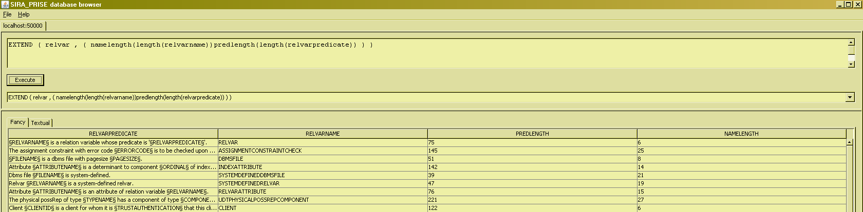
The mechanics of the EXTEND operator are that the extend expressions are evaluated for each tuple from the input relation. The extend expressions can therefore contain references to attributes of such a tuple in the input relation :
It is also possible to include more than one extend expression :
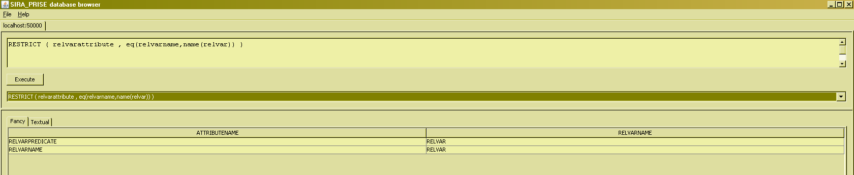
RESTRICT
An example of a question, the answer to which can be given using RESTRICT, is "List all the attributes of the relvar named 'RELVAR'") :
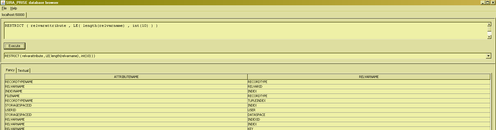
The restrict condition is obviously not restricted to just equality tests on some attribute of the input ("List all the attributes of relvars whose name's length is less than or equal to 10") :
It is beyond the scope of this treatment to go in detail on all the scalar operators that are available for use in restriction conditions and extend expressions. For more detail on that, see the javadoc for the typeimplementations package.
Ordering results
Recall from the first JOIN example, that "lines are scattered all over the place", or iow, tuples seem to appear in completely random orderings. This is in keeping with the principle that there is no inherent ordering to the tuples that appear in a relation. Well, all that might be so in theory, but what can I do if I want to impose an ordering on the tuples in my result sets ? Must I really code the ordering myself on the client side of things ? What if there simply is no code on the client side ? To meet such desiderata, SIRA_PRISE allows to specify a set of attributes for the ordering :
The tuples are now dislayed in ascending order of the specified attribute, the errorcode number. Specifying descending order is currently still unsupported (sorry). Specifying multiple ordering attributes, in descending order of importance, is supported :
Advanced relational algebra operators
This section will provide detail on the more advanced operators and constructs supported in SIRA_PRISE. You can skip this and revisit later if you just want to get going, doing some basic queries. Operators and constructs explained in this section are relation transforms, grouping and ungrouping, relational division, transitive closure, symmetric difference, relation aggregations and summaries, and relation value selectors.
TRANSFORM
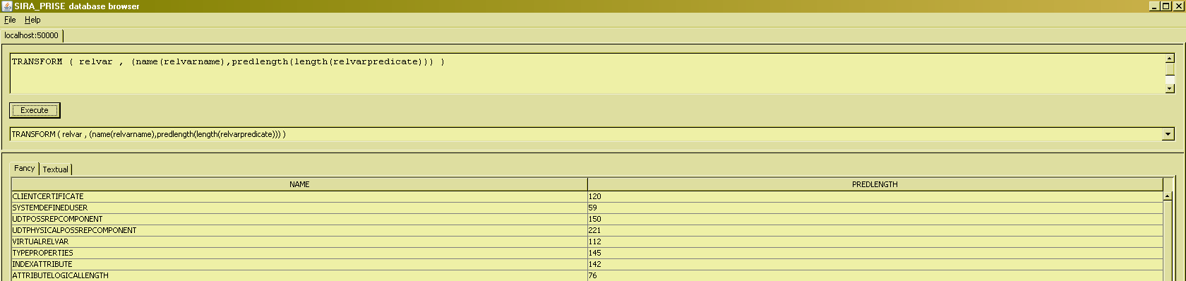
In the context of EXTEND expressions, one scenario that often pops up is that you need an attribute of an input expression to compute the value of an extend expression, and after that is done you can project away the "input" attribute. Always having to explicitly write out the EXTEND and PROJECT invocations, is tedious. A shorthand is made available that combines both operations into one : TRANSFORM. The syntax of a TRANSFORM invocation closely resembles that of EXTEND, with the following differences in defined behaviour :
- Unlike EXTEND, not all attributes of the input expression will be retained in the resulting relation. Instead, the resulting relation will have only the attributes mentioned in the transform definitions list.
- The corresponding expression is optional, not mandatory. In that case, the named attribute must be an attribute of the input relation, and it means, "just copy the values for this attribute into the resulting relation".
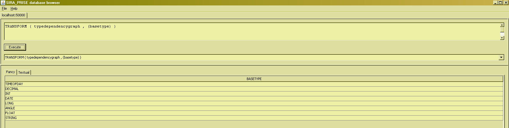
Thus, we can write all projections as a transform : ("transform the value of the typedependencygraph relvar in such a way that only the 'basetype' attribute is retained, and no attributes are 'added' to the result")
GROUP
Recall from the example where keys were joined to their constituent attributes, that "the lines concerning the same relvar, or even the same key, were "scattered all over the place". One way to overcome this, is to impose an ordering to the tuples returned. Another way is to use the GROUP operator to "group together" the information that is contained in multiple tuples, into one single tuple. That one single tuple will have at least one attribute that is relation-valued, i.e. the values appearing for that attribute in the resulting relation are themselves relations, consisting themselves of possibly multiple tuples (and/or possibly multiple attributes).
An example of such an invocation of GROUP to "group together" all the attributes of a key, is :
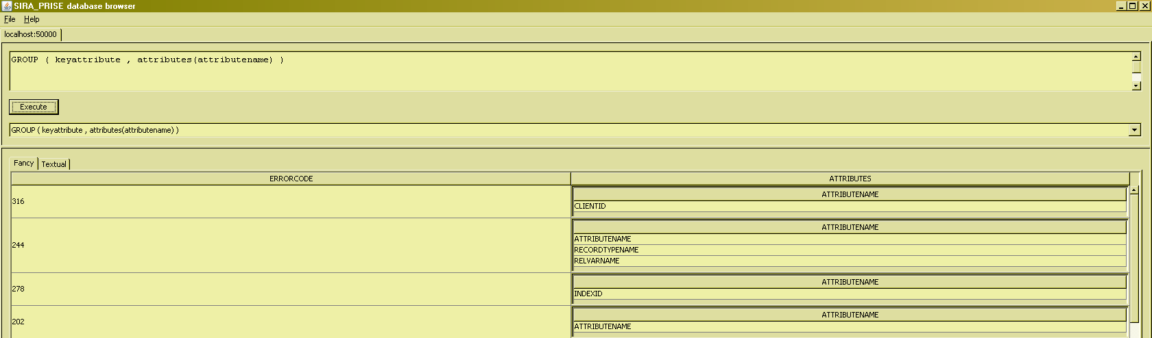
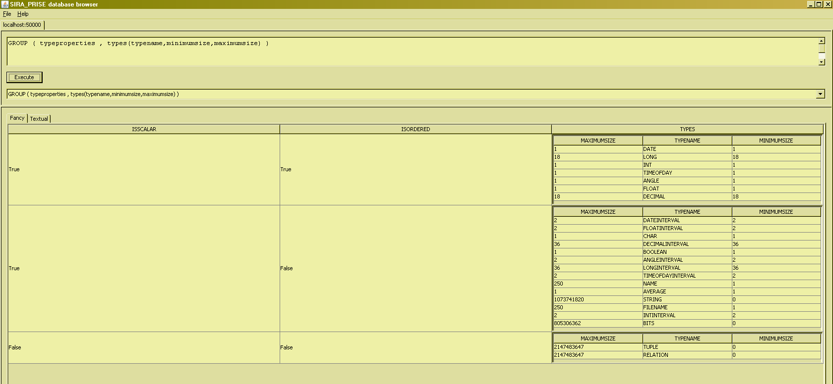
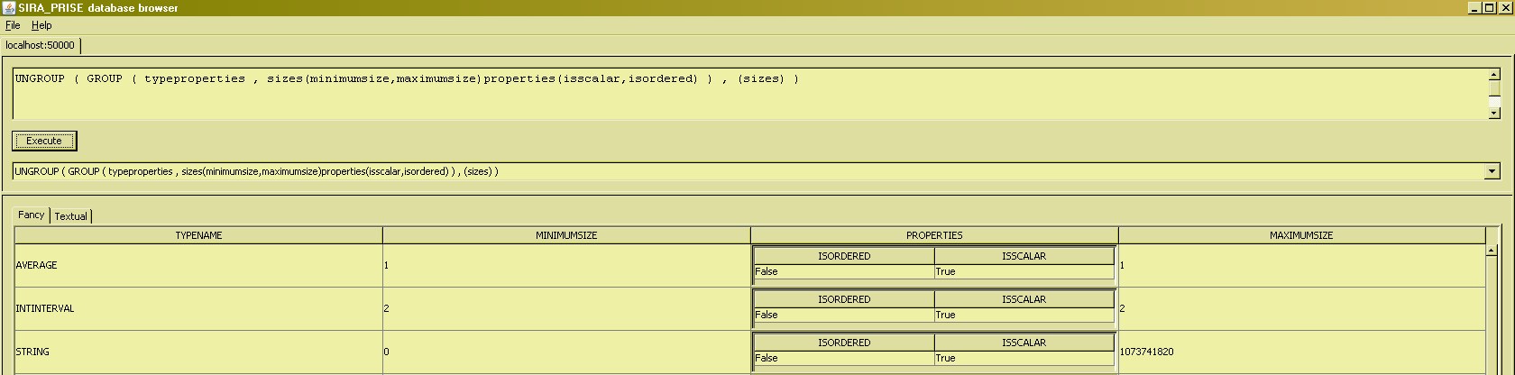
In the example given, the relation-valued attribute (RVA for short) is of degree one, because only one attribute of the input relation was mentioned in the grouping definitions. It is perfectly possible, however, to use GROUP to create RVA's of any arbitrary degree : just list all the input attributes you wish to be grouped together, e.g. as in the following -somewhat contrived- example :
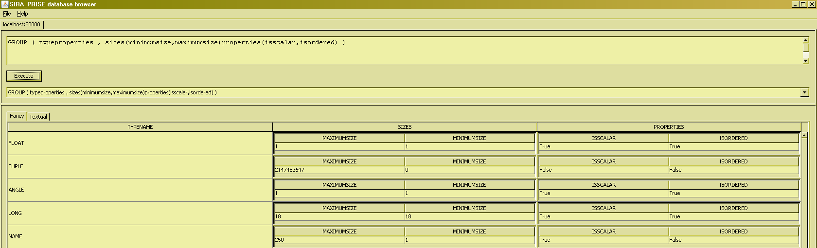
It is also possible to use GROUP to create more than one RVA :
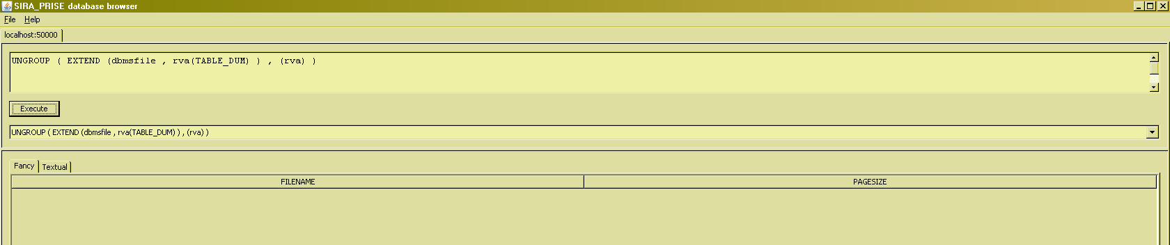
UNGROUP
The inverse operation of GROUP is called UNGROUP. UNGROUP takes a relatinal expression and a set of attribute names, all of which must be relation-valued in the input. A bit predicatbly, an UNGROUP invocation can "reverse" relations such as those produced by GROUP, to the input they were created from :
If an RVA value is the empty relation, then the tuple in which it appears will not give rise to a tuple being present in the UNGROUP result :
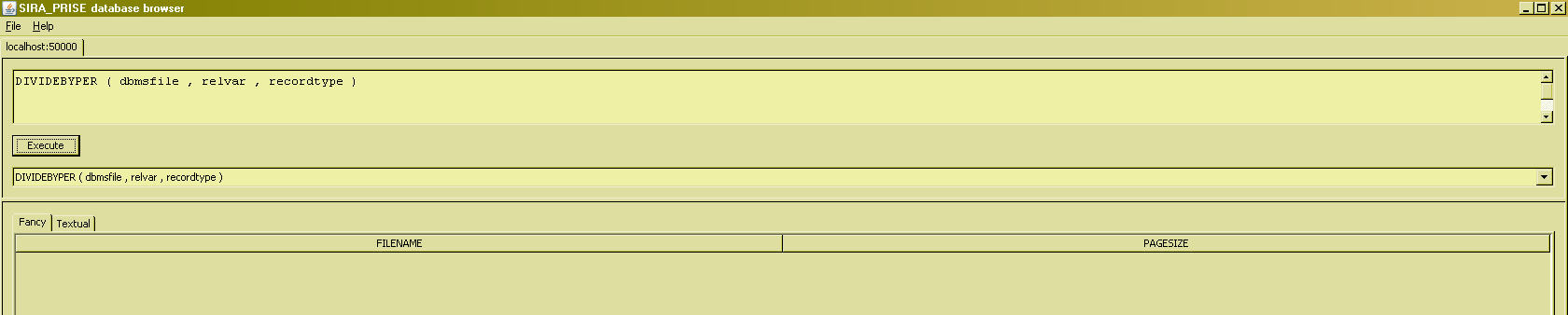
DIVIDEBY
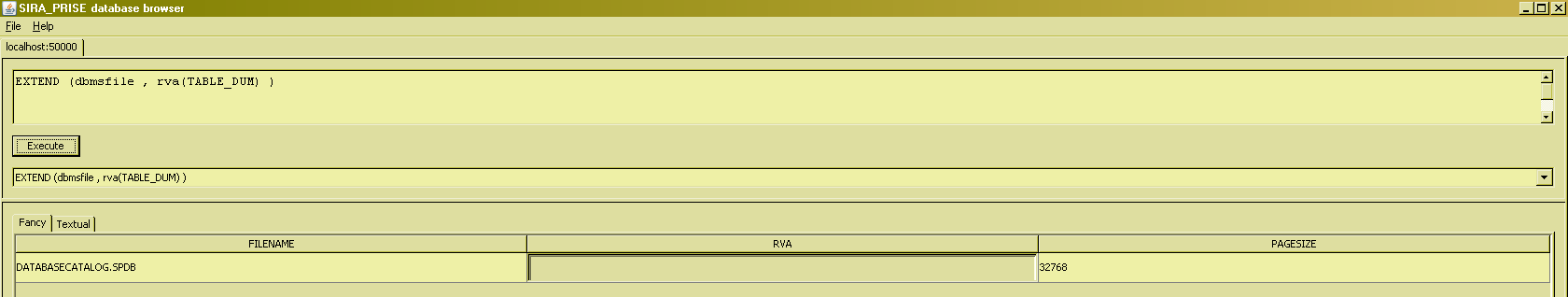
SIRA_PRISE also supports a relational division operator. "A" relational operator, indefinite article, because the operation of relational division has a very long history behind it, and many versions of it have been defined over the years. Recanting that entire history is beyond the scope of this document. Those interested can find an excellent account of this history in, a.o., "Database Explorations", chpt. 12. The relational dividsion operator serves the purpose of answering queries of the general nature "get me the X's that ... all Y's". In there, X's and Y's are types of things about which the database maintains information, and the ... is a possible relationship between X's and Y's, where the database also maintains information about [instances of] that relationship. For example, X could be "Suppliers", Y could be "Parts", and the ellipsis could be the relationship that "Suppliers supply Parts in certain set quantities". In the following examples, the X's and Y's will be "Relvars" and "Physical Storage Files", and the relationship between them is that a Relvar can have an associated RecordType, which is physically stored in a File.
The first example illustrates how to answer "Get all the relvars that have an associated record type in all existing files" :
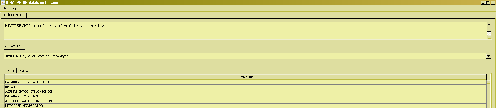
Getting the arguments in the "right" order is the trickiest part. That "right" order is : the X's first, then the Y's (the one that holds the things mentioned after the 'all' in the natural-language formulation of the query, in this case 'all existing files') , and the intersection relation last (the one that holds the instances/appearances of the relationships between X's and Y's). For those familiar with it, observe how this is different from Codd's original divide operator, using which one would have to have written something like 'DIVIDE <intersection relation> BY <Y's>.
If the query were instead, "Get the files that hold a record type for all relvars", then the first two arguments would have to change places :
The result should indeed be empty, since there exists a relvar or two that have no associated record type at all, making it obviously impossible for any file to "hold a record type for all relvars".
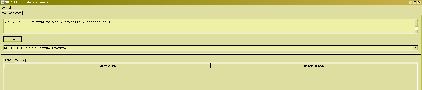
The following examples are to explain/demonstrate the behaviour of the division operator in the face of empty divisors. The first one answers the question "What are all the virtual relvars that have an associated record type in all files ?". And since virtual relvars have no record type associated with them at all (which is precisely what makes them 'virtual'), we can expect this query to produce an empty result :
But if we change the question to "What are all the virtual relvars that have an associated record type in all files whose page size is >50000 ?" (the point being that there are no such files, at least not immediately after you installed the system), then we get this :
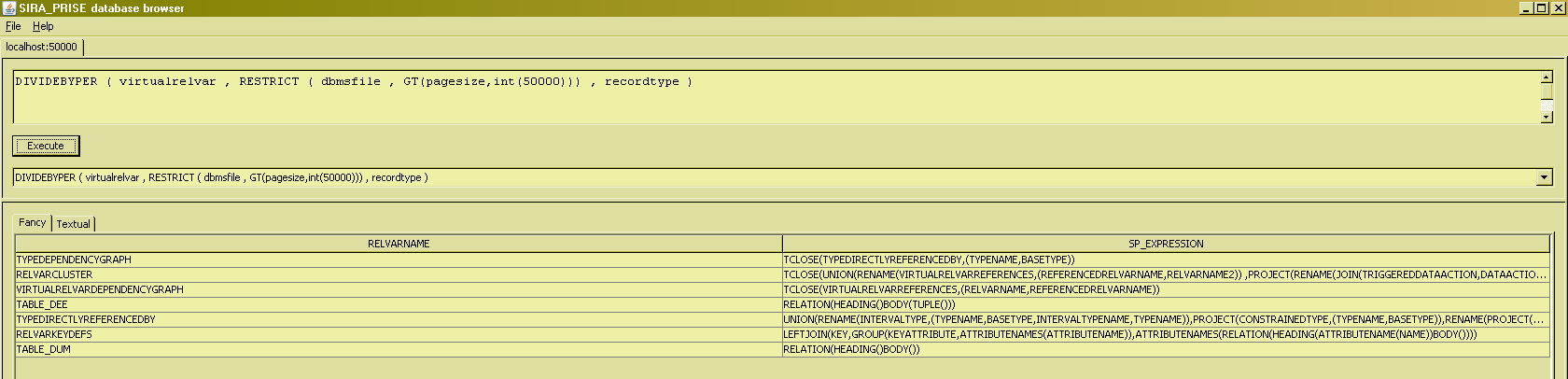
This (simply all virtual relvars) is indeed the correct result, since there does not exist a virtual relvar such that there exists a file having a page size >50000 and such that that virtual relvar does not have an associated record type in that file. With sincere apologies for all those confusing negations, but there doesn't seem to be a better way to explain ...
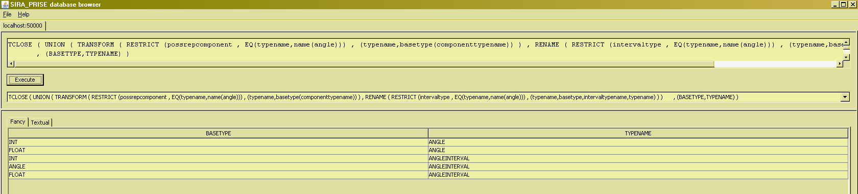
TCLOSE
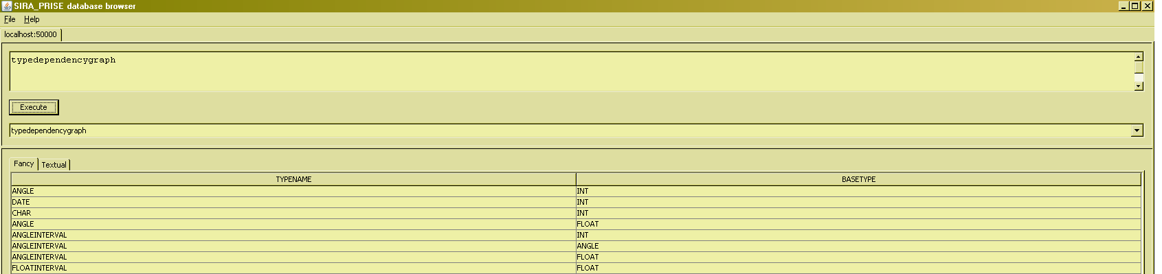
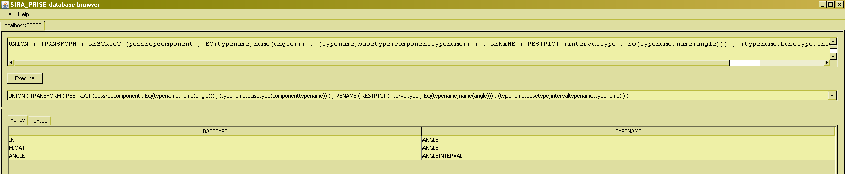
The transitive closure operator is used essentially for dealing with graphs. We assume that you are familiar with the essentials of graph theory, and the usual way to represent graphs in relational structures : as a set of connections ("edges") between nodes ("vertices"). Recall that some examples used so far were based on a relvar named 'typedependencygraph'. This (virtual) relvar defines which types are dependent on which other types for their definition. There can be many reasons for such a dependency, but for the present purpose of explaining the TCLOSE operator, we will just focus on two of them :
- Another type might be needed for the definition of some type, because that other type is needed to express the value for a possrep component of a value of the dependent type,
- Interval types can only be defined if a type exists that can express the boundary values of [values of] the interval type at hand.
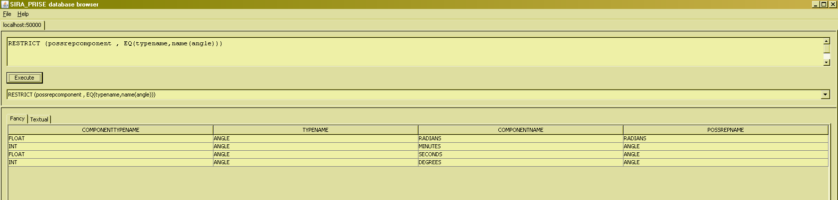
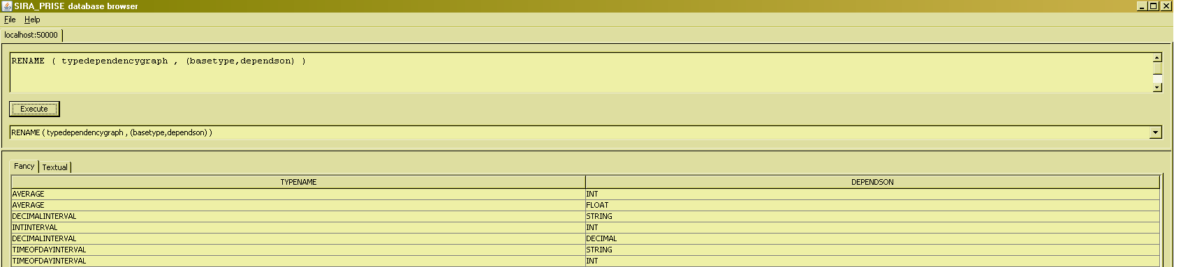
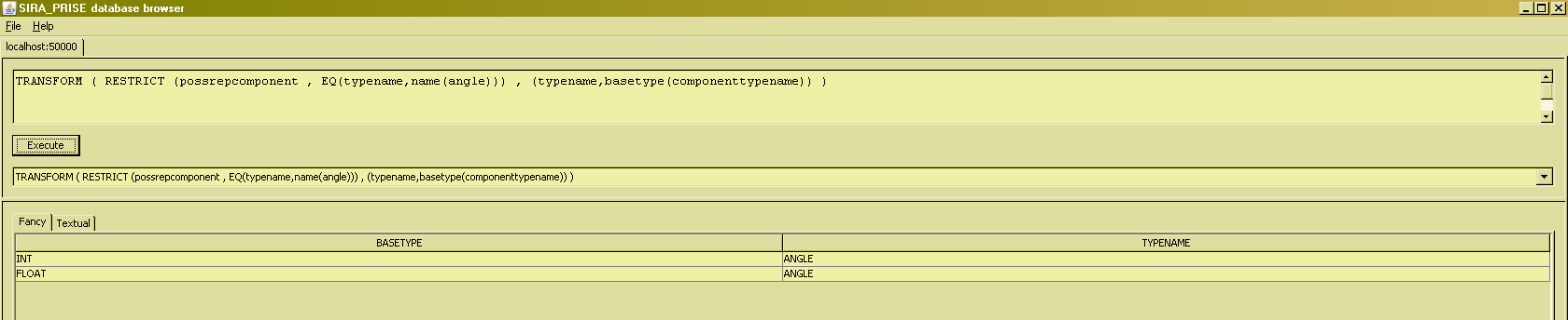
Using the ANGLE possrep, it reveals that we need a type INT to be able to express the degrees and minutes portion of any angle value, and also that we need a type FLOAT to be able to express the seconds portion of any such value. Using TRANSFORM, we can therefore express the fact that type 'ANGLE' depends on types 'INT' and 'FLOAT' :
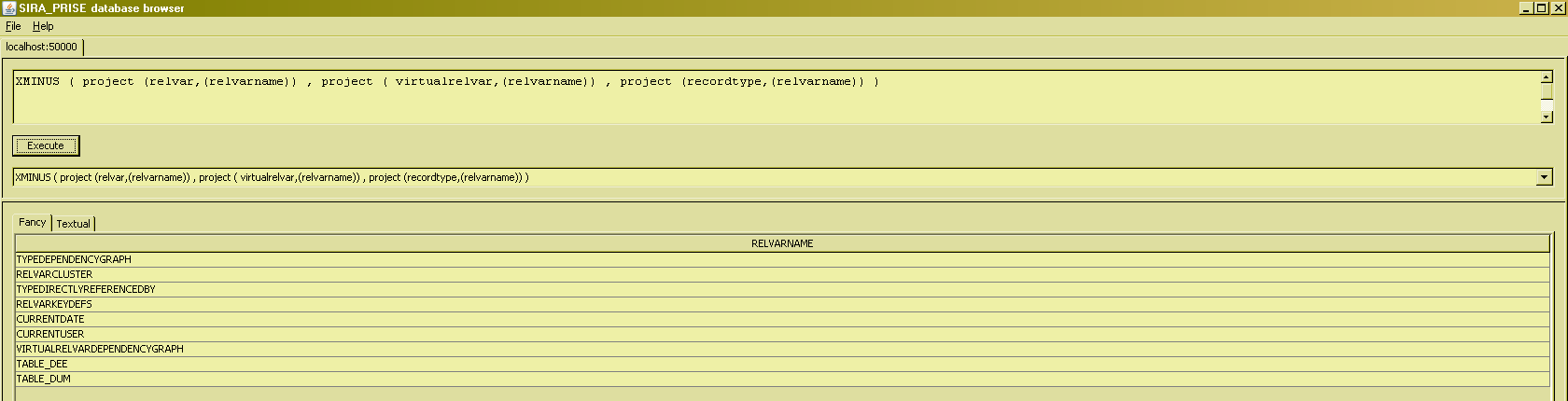
XMINUS (symmetric difference)
The symmetric difference of two relations is defined as the union of their mutual differences. That is, XMINUS(R1,R2) is defined to be equivalent to UNION(MINUS(R1,R2),MINUS(R2,R1)). There is little more to be said about it except that the operator happens to be associative, and that it is thus possible to invoke symmetric difference with more than just 2 arguments (just so long as all arguments have the same heading, of course, and on another twist, just so long as you don't try and make much sense out of the results such an associative invocation produces) :
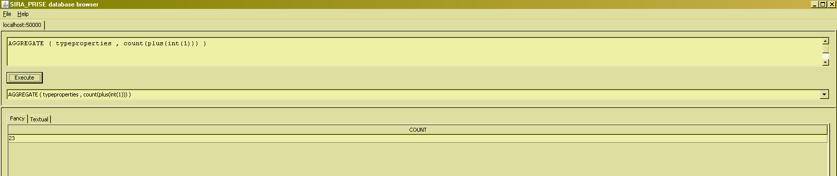
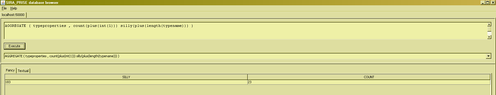
AGGREGATE
The AGGREGATE operator is an additional operator in comparison to TTM. It is much more basic in its operation in comparison to TTM's summarize (thus also less functional), and is in fact a "building block" on which the implementation of SIRA_PRISE's SUMMARIZEBY operator relies. The rules for aggregate are as follows :
- The input is exactly one relation, plus a list of <AggregationDef>s.
- Each <AggregationDef> has the structure "<AttributeName>(<OperatorName>(<Expression>))"
- AGGREGATE always produces a singleton relation as its output.
- The degree of that produced relation will be equal to the cardinality of the list of <AggregationDef>s. Obviously, duplicate attribute names cannot be specified.
- <AttributeName> specifies the name of an attribute in the relation produced by AGGREGATE.
- <OperatorName> must be the name of an aggregation operator on the type of <Expression>, and whose return type is also the same. An operator is an aggregation operator if and only if it is both commutative and associative (obviously, the operator implementation must declare these characteristics for SIRA_PRISE to be aware of this). Note that it is not sufficient to be just associative. String concatenation is an example of an operator that is associative, but not commutative. Therefore string concatenation cannot be considered a valid aggregation operator.
- <Expression> must denote a valid expression of the type that the associative operator can act upon. The only allowable variables in this expression are attribute references to the relation that is being aggregated.
- The value for <AttributeName> in the (single tuple in the) resulting relation, will be equal to the value produced by the invocation of the specified operator, using as arguments all the values that appear for <Expression> in the relation that is being aggregated.
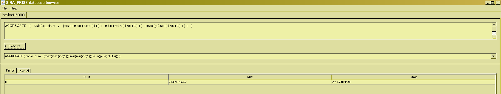
Aggregate thus provides a, perhaps somewhat clumsy, substitute for operators such as TTM's COUNT(<Relation>) :
Some kinds of aggregation require a somewhat special approach, e.g. to compute averages from a set of observations :
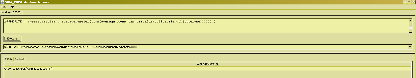
Observe the following points :
- The operator name is PLUS (a plus operator that operates on "pairs" (n,v) and (m,w), returning a "pair" (n+m , (n*v+m*w)/(n+m) ) )
- The expression aggregated is a value selector of type AVERAGE
- That value selector selects values with two components, an observation count and an observation value
- The observation count component is of type INT
- The observation value is of type FLOAT
- Getting the 'FLOAT' value for the type's name's length, involves invloking TOFLOAT operator on an integer argument.
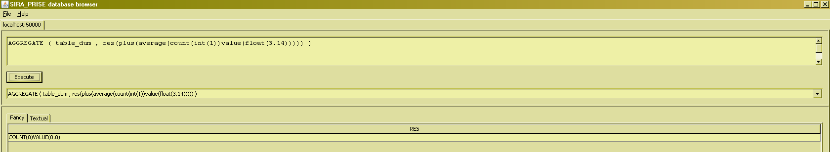
Cumbersome perhaps, but it works, and at least it is explicit about the observation count, also in the following case :
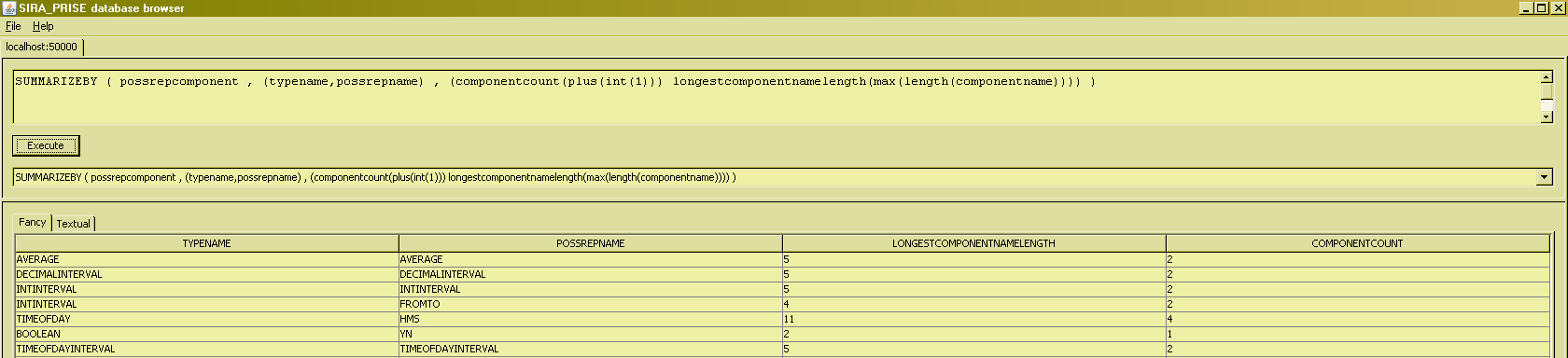
SUMMARIZEBY
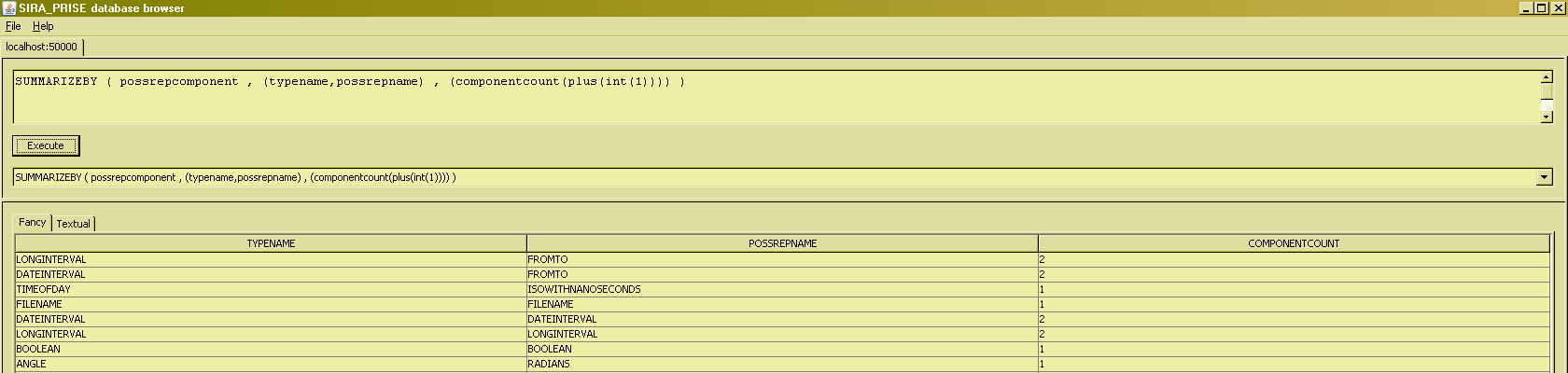
Whereas AGGREGATE always returns aggregations over an entire relation, SUMMARIZEBY can do the same over "partitionings" of relations, thus resembling more to the SQL type of aggregate queries. Compared to AGGREGATE, SUMMARIZEBY takes an extra argument, which is the "grouping key" for the summary. The following example shows the query for "Get the count of components of each defined possrep of a type" :
As with AGGREGATE, multiple summaries can be built "in one and the same go" :
For the fun of it, you can check for yourself if SIRA_PRISE supports the edge case of "no grouping attributes at all". The grouping key must consist exclusively of attribute names of the input expression. Grouping on the result of arbitrary expressions (e.g. SUBSTR (relvarname , 1 , 2) is not
supported. If such groupings are needed, extend or transform the input expression appropriately such that the values of such "grouping key expressions" are contained as an attirbute value in the result.
Relation Value Selectors
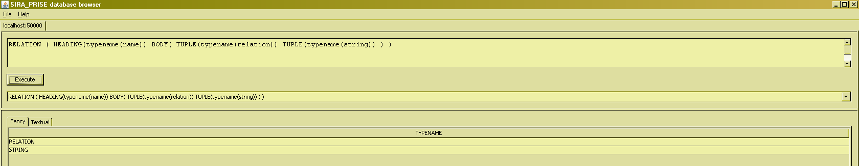
When writing a relation value selector, the system needs to be informed of the heading (the relation type) of the value selector and of the body (the set of tuples) of the value selector. Simply inferring the heading from the body is not always an option, and is currently not supported. Thus, a relation value selector has the general syntactical structure RELATION(HEADING( ... )BODY( ... )).
The HEADING portion names the attributes in the relation, with the attribute's type in parentheses. E.g. for (a heading consisiting of) an attribute named 'typename' which is of type 'name' : RELATION(HEADING( typename(name) )BODY( ... )), or for a relvar with the same heading as the 'relvar' relvar (used in the very first example of this guided tour) : RELATION(HEADING( relvarname(name) relvarpredicate(string) )BODY( ... )).
The BODY portion contains all the tuples that will be part of the relation body, in the syntax TUPLE( ... ) TUPLE ( ... ) ...
The ellipsis inside those TUPLE( ... ) constructs denote value selector expressions for all the attributes listed in the heading. Thus, a complete relation value selector looks something like :
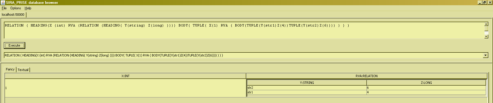
Since relations in general can have attributes that are themselves relation-valued, it must also be possible to write relation value selectors for them. This possibility obviously affects what there is to write in the HEADING() and BODY() portions of the value selector. The following will illustrate the way to write a value selector for a relation of degree two, with attributes X and RVA, where RVA is itself relation-typed, also of degree two, with two attributes Y and Z.
- In the HEADING portion, we obviously have to include the declaration for the X attribute, so we begin with HEADING (X (int) )
- We obviously also have to include the delcaration for the RVA attribute, which is of type RELATION, so we get HEADING (X (int) RVA (RELATION) )
- But saying that RVA is of a relation type obviously isn't sufficient, we will also have to specify the heading for that relation type. We include that in parentheses behind the RELATION keyword to get : HEADING (X (int) RVA (RELATION (HEADING( Y(string) Z(long) ))) )
- In the overall construct, that gets us RELATION ( HEADING(X (int) RVA (RELATION (HEADING( Y(string) Z(long) )))) BODY( ... ) )
- In the TUPLE(...) portions of the BODY() specification, we will have to provide value selector expressions for both X and RVA. So we'd need something like, e.g., TUPLE( X(1) RVA ( ... ) )
- Observe how the literal for the X value in this tuple, lacks the type specification that would otherwise be needed, as in INT(1). This is possible because the value selector already knows X to be an INT, from the heading declaration.
- Likewise, the overall value selector already knows RVA to be of a RELATION type, and its specific heading. Thus we don't need to duplicate the RELATION(HEADING()) part of the value selector when specifying a value for RVA, and we can suffice with just the BODY() part for each value of RVA : RVA ( BODY(TUPLE(Y(str1)Z(4))TUPLE(Y(str2)Z(6))) ).
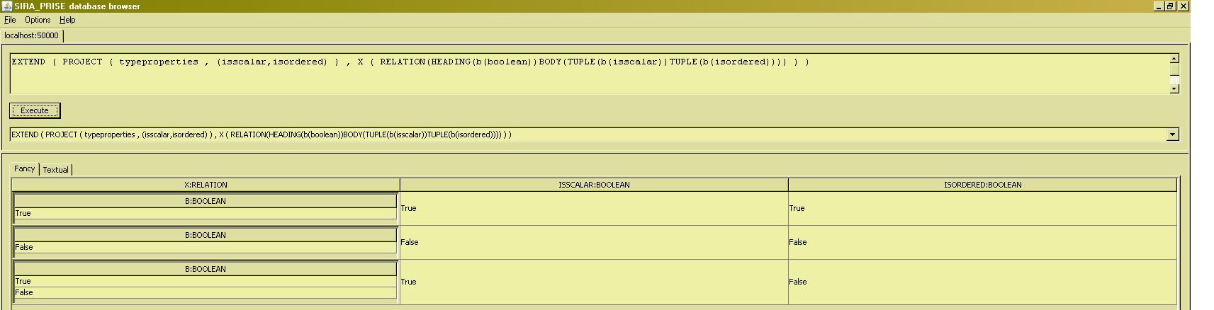
Since the expressions for selecting the attribute values in the tuples in the body, can be just any expression in general, these attribute value selectors can contain references to attributes that are in scope (attributes 'isscalar' and 'isordered' in the next example), or references to database relvars (subsequent example) :
And this example uses database relvar references to specify the value of (relation-valued) attributes in the resulting relation :
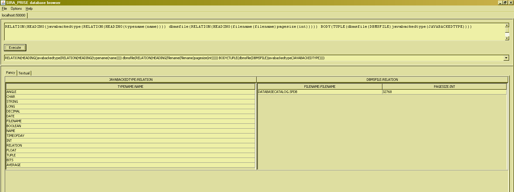
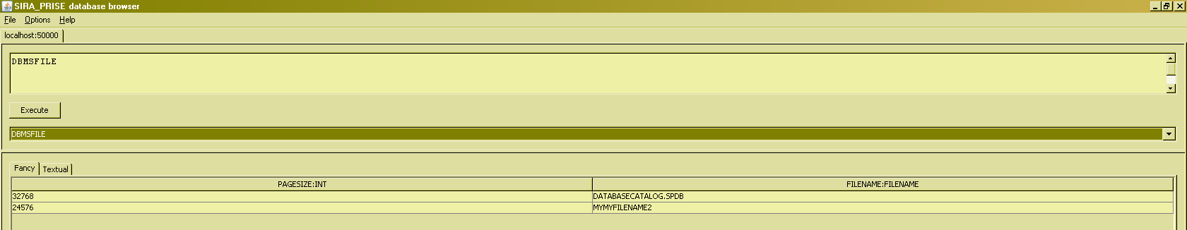
(Readers who are very familiar with the concepts of TTM might recognise here the concept of a database [value] being a tuple [value], where the attributes are all relation-valued and their names correspond to the relvar names as seen in the more traditional view of a database. The given example being a case of a database with two relvars, DBMSFILE and JAVABACKEDTYPE, the former of degree 2 and the latter of degree 1.)
As the examples have shown, writing relation value selectors can be quite tedious. A further "shorthand" is available for writing relation value selectors of a relation type that is the same as the relation type of an existing database relvar. In those cases, a relation value selector can be abbreviated to just the relvar's name, plus the TUPLE() value selectors :
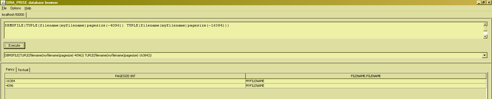
Observe from this example that the only inferences made from the database relvar, are about its heading (its relation type). Constraints on the database relvar in this example prohibit negative page sizes, and prohibit nonunique filenames, but these constraints do not carry over to a relation value selector that uses this syntactic shorthand.
Defined virtual relvars can equally well be used in this syntactic shorthand (perhaps try and explain the -correct- results as an exercise) :
Updating databases
This section will briefly introduce the syntax for SIRA_PRISE's database update commands. The examples here will illustrate update commands using the catalog for a database. And although defining new databases is indeed done through updating the catalog, note that this section is not intended as a guide for "how to design and define complete databases". The better place to look for that info is the catalog reference.
Adding information to a database
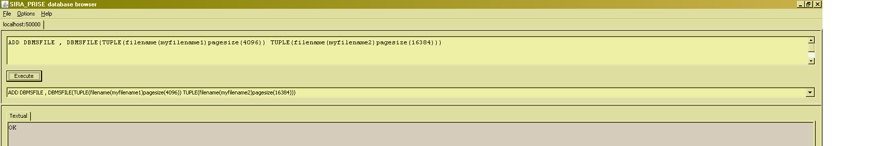
The basic way to add information to a database, is to issue an ADD or ASSERT command. Both name the target relvar (which is not allowed to be a virtual relvar - SIRA_PRISE has no view updating), and a relational expression to compute the tuples to be included in the current value of the named target relvar. The relation type of that relational expression must obviously be the same as the relation type of the target relvar. The difference between ADD and ASSERT is that ADD does not allow any tuple-to-be-included to appear already in the current value of the target relvar (ADD is really ADD : tuple t is not yet there but must be, hence must be added), whereas ASSERT merely has the effect to assert (hence the name) that any tuple-to-be-included will appear in the value of the target relvar after the update, irrespective of whether it already does or not. The "anatomy" of an ADD/ASSERT command is simply <keyword> <targetrelvarname> , <relationalexpression> :
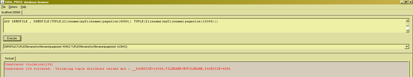
An example of an acceptable update would be :
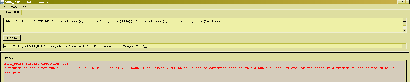
Issuing the same command again will yield :
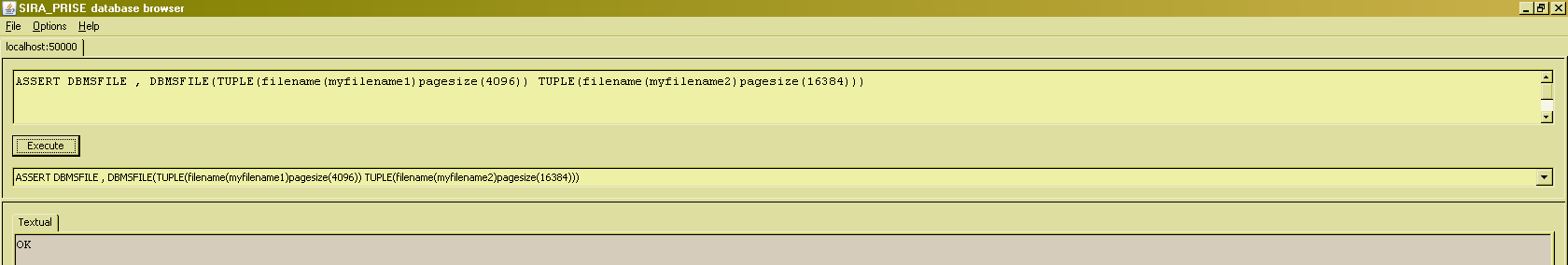
Whereas issuing the ASSERT form of this update will be accepted (even if it amounts to a complete no-op) :
Deleting information in a database
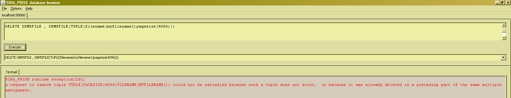
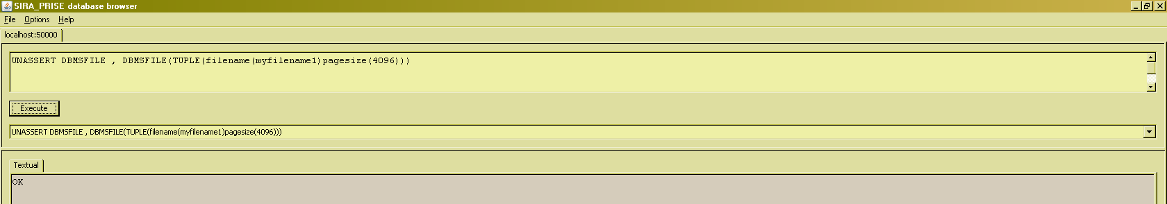
The basic way to delete information from a database, is (three guesses allowed) to issue a DELETE or UNASSERT command. Both name the target relvar (which is not allowed to be a virtual relvar - SIRA_PRISE has no view updating), and a relational expression to compute the tuples to be excluded from the current value of the named target relvar. The relation type of that relational expression must obviously be the same as the relation type of the target relvar. The difference between DELETE and UNASSERT is that DELETE does not allow any tuple-to-be-excluded to be already absent from the current value of the target relvar (DELETE is really DELETE : tuple t is effectively present but must not be, hence must be removed) whereas UNASSERT merely has the effect to assert (hence the name) that any tuple-to-be-excluded will not appear in the value of the target relvar after the update, irrespective of whether or not it already does. The "anatomy" of a DELETE/UNASSERT command is, predictably, simply <keyword> <targetrelvarname> , <relationalexpression> :
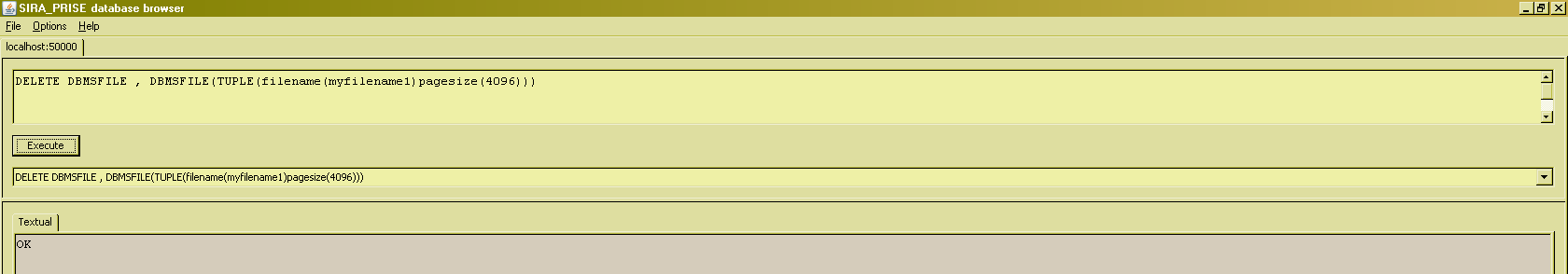
Issuing the same command again will yield :
Whereas issuing the UNASSERT form of this update will be accepted (even if it amounts to a complete no-op) :
Updating information in a database
The following is an example of an update command :
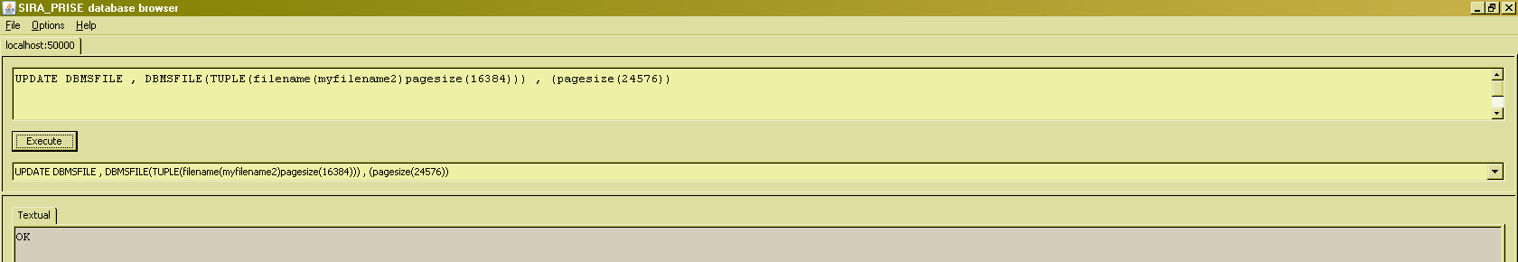
Its "anatomy" is as follows :
- The name immediately following the UPDATE keyword names the target relvar (DBMSFILE)
- Following that, is a <relational expression>, defining which tuples will be "subjected" to the update. The relational expression is required to have the same relation type as the target relvar, and all tuples in this expression are required to be present in the current value of the target relvar (this can be ascertained by writing the expression as being a restriction on or a join with the target relvar itself). In the example, the expression is a relation value selector holding one tuple.
- Following that, comes a list of <update expression>, defining what the replacing values will be for the tuples that are subjected to the update (i.e. what the replacing tuples will be for the tuples in the foregoing <relational expression>. In the example, the update expression list specifies that in all tuples "subject-to-update", the replacing value for the pagesize attribute will be (the literal) 24576.
The overall effect (on the current value of its target relvar) of the UPDATE is that first, all tuples that are subjected to update, are removed from the current value of the target relvar, and subsequently, all the computed "replacing tuples" are added. Note that this can result in a no-op. Thus, UPDATE will always have the same effect on the current value of its target relvar, as a certain DELETE-then-ADD sequence, combined together in a single operation.
UPDATE will not allow two "replacing tuples" to be equal to one another. This means that it is not possible to issue an UPDATE such that two existing (and thus distinct) tuples get "mergered together" and replaced by only one.
UPDATE does not limit the <update expression> list to affect only nonkey attributes. This means it is possible to use an update to change key values :
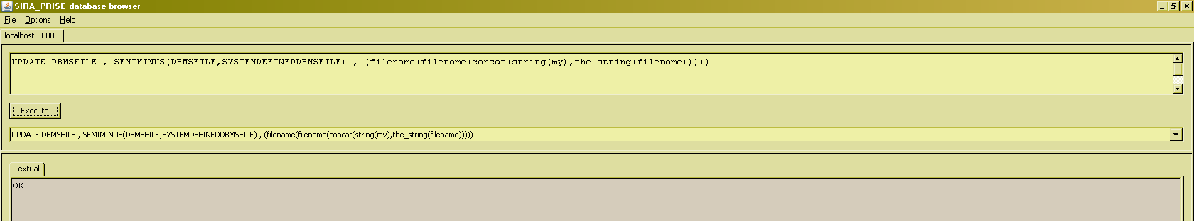
The anatomy of the given example :
- The target relvar is the DBMSFILE relvar
- The affected tuples are the ones that appear in the value of the SEMIMINUS expression, which basically means "all defined files except the catalog"
- The only afftected attribute is the 'filename' attribute (the outermost ' filename( ' construct)
- Its replacing value will be computed by the value selector provided for that attribute (the second ' filename( ' construct, this time denoting a value selector invocation for the concerned attribute's type, which happens to have the same name as the attribute)
- The argument to that filename value selector, is itself an invocation of the string concatenation operator, the arguments to which are (a) the string literal 'my', and (b) the string rendering of the value of the 'filename' attribute of the tuple that is "subject to update".
Also note that, as the foregoing example demonstrated, the <update expression>s can hold references to attributes of (the "subject-to-update" tuples of) the target relvar. mymy :-)
Multiple Assignment
Many times, applicable constraints put the database updater in a chicken-and-egg kind of stalemate position. A typical example from a personnel database :
- Each employee must be assigned to a department
- Each department must be assigned a manager
- and that manager must be a known employee
Starting with an empty database, you cannot insert the first employee, because there are no departments yet to assign that employee to, and you cannot insert the first department because there are no employees yet that can be assigned as the manager of that department.
Allowing database users to start fiddling around with the constraint check times can get quite messy, and this is why TTM defines the concept of multiple assignment, which is indeed supported by SIRA_PRISE.
The applicable chicken-and-egg stalemate from the SIRA_PRISE catalog that we will be using in the examples is the following :
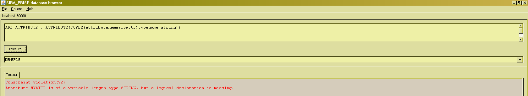
- Types can be declared to be of "variable-length", or of "fixed-length" (one example of a variable-length type is type STRING).
- Attributes are required to be [declared to be] of a type.
- If an attribute's type happens to be variable-length, then a logical length must also be defined for that attribute.
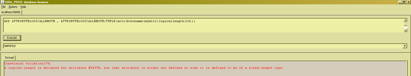
- All logical-length declarations for attributes must be for known attributes.
- We cannot just declare attributes of type STRING, because there will be no logical length declaration for them,
- and we cannot register the logical-length declaration, because there will not yet be a corresponding attribute declaration :
and attempting to declare the logical length :
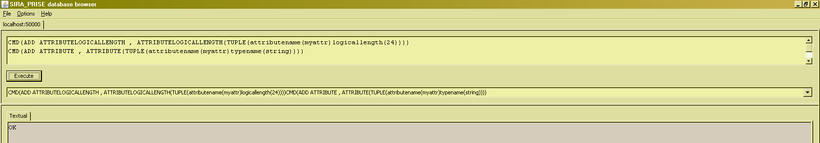
- There are no inherent restrictions on the mixture of ADDs, DELETEs and UPDATEs that constitute a multiple assignment. For example, in certain cases constraints micht be such that introducing a key value in one relvar, will require removing that value from another one "at the same time".
- There are no inherent restrictions as to the number of times a relvar can be mentioned in the distinct "individual" portions that constitute the multiple assignment. In theory, the rules as laid out in TTM apply, but at present it turns out to be very hard to implement those rules for the full 100%. But at any rate, overusing this particular feature can easily lead to unexpected behaviour, even if that bebaviour complies fully to the TTM rules, so overusing this feature is quite strongly discouraged.